
About the Dashboard
What sites are in the program?
Participants in WastewaterSCAN are municipal treatment plants in the United States that serve >10,000 people, with some plants serving up to around 4 million people. The goal of analyzing wastewater at this level is to get a picture of infectious disease occurrence at a community population scale. Sampling at this scale covers a population large enough that positive results for a disease won’t be associated with individuals.
To learn more about the WastewaterSCAN program please visit: https://www.wastewaterscan.org/en/about
What are you testing for?
WastewaterSCAN tests samples of solids from municipal wastewater for targets associated with infectious diseases. The concentration of these targets in wastewater is associated with the occurrence of the related disease in the community, and changes in the concentrations of these markers in wastewater over time tell us about changes in the rates of disease in the community. WastewaterSCAN only tests for analytes that are related to infectious diseases. All of our methods are published and open, and are linked in sections below.
As of October 2025, we are testing for the following pathogens:
- Respiratory pathogens: SARS-CoV-2 using a conserved target on the N gene, Influenza A (IAV), H1 + H3 + H5 influenza markers,Influenza B (IBV), Respiratory Syncytial Virus (RSV), Human metapneumovirus (HMPV), Enterovirus D68 (EVD68)
- Gastrointestinal pathogens: Norovirus GII, Rotavirus, and Human adenovirus group F
- Other pathogens of concern: Candidozyma auris (C.auris), Hepatitis A (Hep A), Measles (wild-type), Mpox clade Ib, Mpox clade II, and West Nile virus (WNV).
We continue to develop tools for monitoring new variants and additional infectious diseases, and may add new targets to this panel over time. We always notify our partners before making any changes to assays and welcome comments on these plans from our partners.
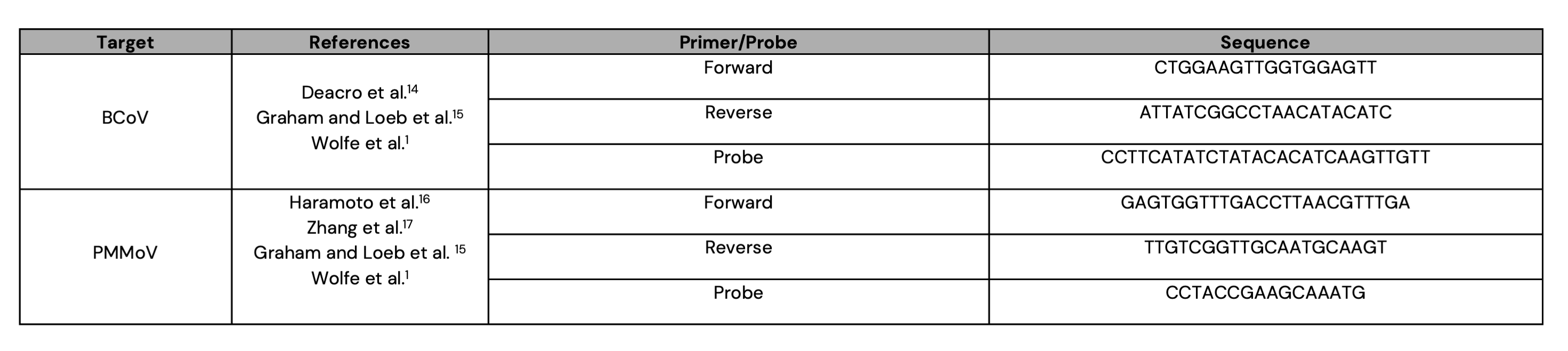
We also test for two controls in every sample. Bovine Coronavirus (BCoV) is spiked into each sample as an exogenous recovery control. Pepper mild mottle virus (PMMoV) is measured in each sample as a normalizing control. PMMoV is a virus that infects peppers and is highly abundant in wastewater. Measuring PMMoV helps us control for variations that occur in wastewater from day to day at a single site and between sites.
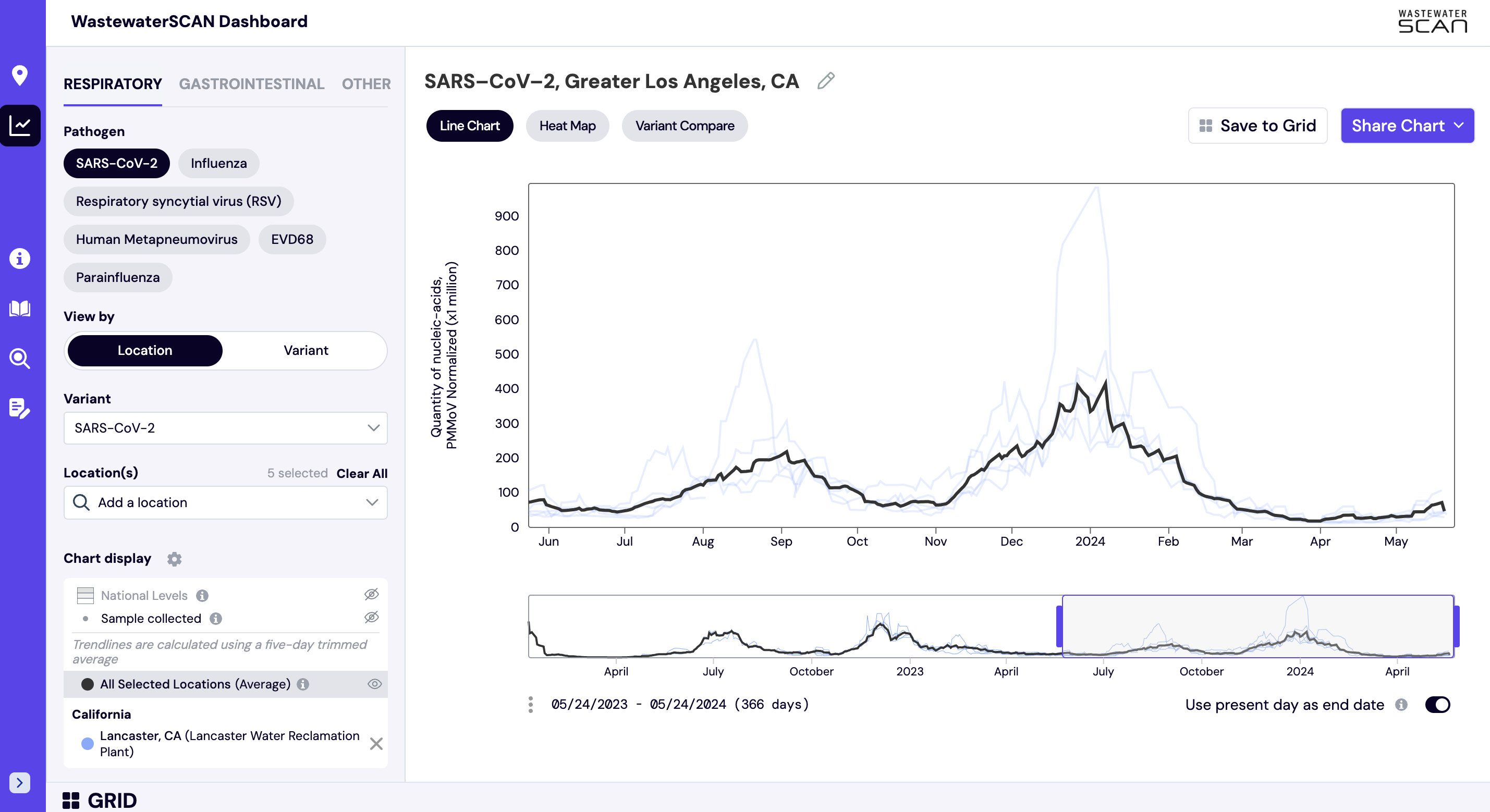
How do I interpret the line charts?
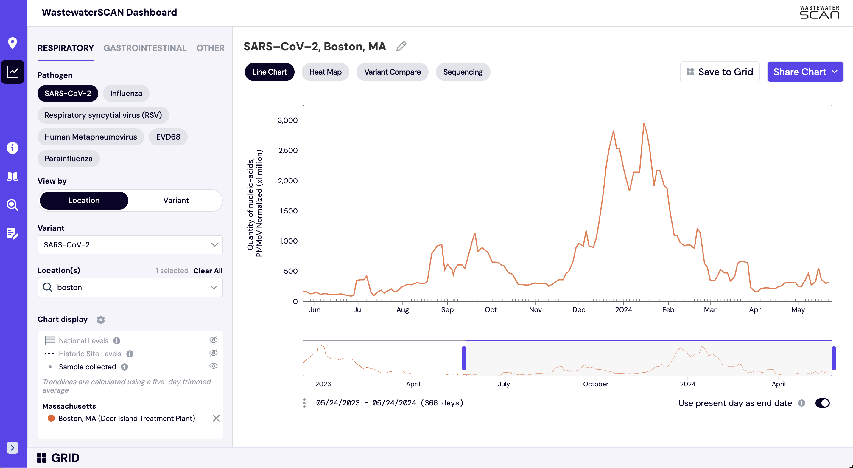
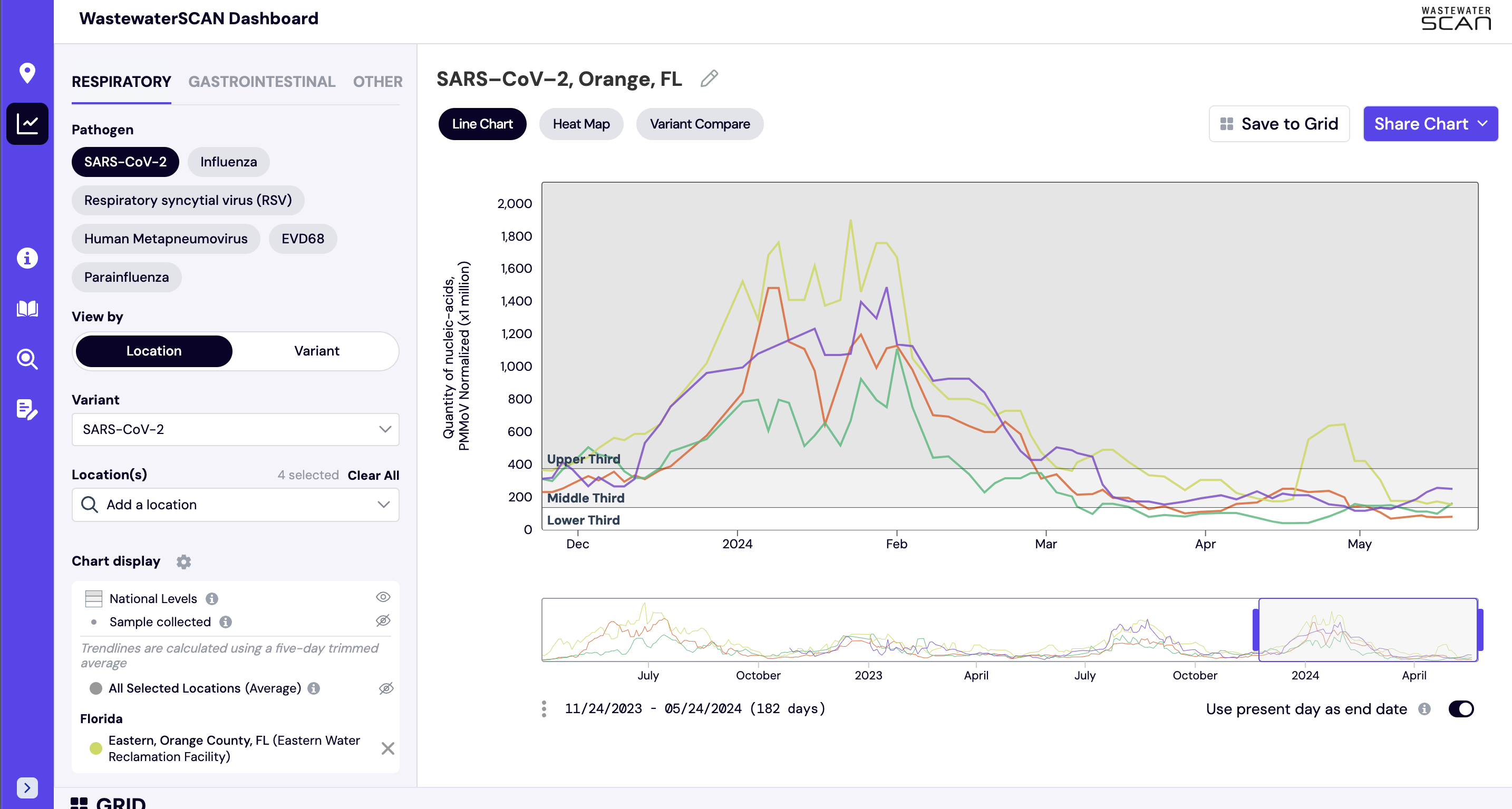
The default view on charts on data.wastewaterscan.org as shown above shows consensus smoothing (5-sample trimmed average) of the selected pathogen concentrations normalized by PMMoV concentrations in the solids. These results are shown on a linear scale and although the target/PMMoV ratio is unitless, it is multiplied by 1 million on the y axis of these plots to make the numbers easier to interpret.
The trimmed average lines shown use 5 consecutive samples, first eliminating the maximum and minimum among the 5 samples and then taking the mean. The smoothing is centered, so the most recent two days of data, it will just use the 3 or 4 values available. This means that as more data is added, the smoothed estimates for the most recent days may update and appear to change.
Normalizing the SARS-CoV-2 genes by PMMoV conceptually corrects for measurement-to-measurement changes in RNA/DNA recovery and fecal strength. This assumes that RNA recovery from PMMoV is similar to that of the target pathogen’s DNA/RNA, and that PMMoV adequately controls for fecal strength of the sample.
The trimmed average normalized by PMMoV is shown as default because the data is most useful for observing trends over time and these strategies are useful to deal with variability in the data and clarify these trends. This document provides additional information about what specific factors lead to variability in this dataset, how these differ from the types of variability we expect in clinical case or syndromic data, and what actions have been taken to mitigate those sources of variability.
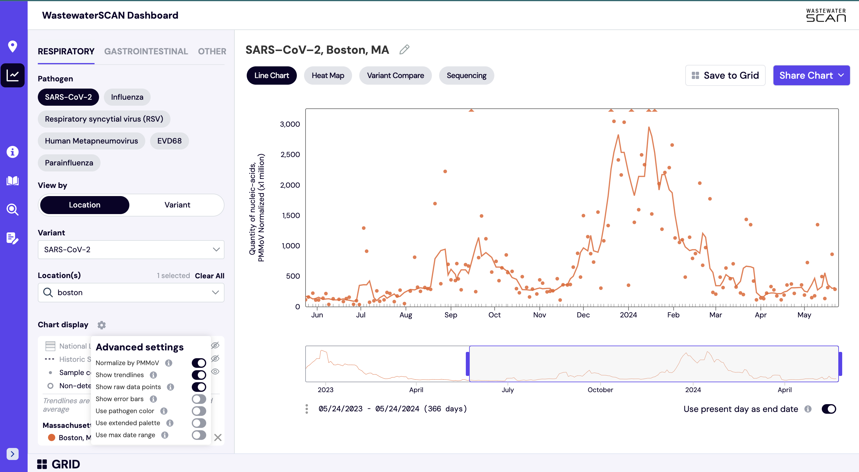
Using the gear menu located on the left side navigation panel, you can see the ‘Chart Display’ settings. In the ‘Chart Display’ you can find the following items:
- Normalize by PMMoV: Show data normalized by PMMoV, a control virus that can help account for changes in wastewater by time and place. The normalized measurements for each target are shown as default view in ‘Chart’ mode.
- Show Trendline: Trendlines are calculated using a five day trimmed average.
- Show Raw Data: Displays individual, unsmoothed for each sample as points.
- Show Error Bars: Shows error bars for the raw data. The errors on each point represent standard deviations (68% confidence intervals) from the droplet digital RT-PCR measurement and include Poisson error as well as variation among 6 replicate wells. Because the errors are Poisson errors they are asymmetrical; so the "top" error bar may be a different length than the "bottom" error bar. The reported ratio error is propagated from the errors on the viral gene and PMMoV gene measurements assuming that the relative error is additive among the numerator and denominator.
- Use Pathogen Color: Shows all sites in the chart in one color, specific to the pathogen being viewed..
- Use Extended Palette: Shows up to ten colors on the chart. If you are viewing up to 10 individual sites, each site can have its own color associated with it.
- Use Maximum Date Range: Extends date range beyond the available data for selected plants and targets.
The normalized measurements for each target are shown as default, but the gear menu can also be used to switch to viewing the concentrations reported in copies of the target per gram of wastewater solids without PMMoV normalization.
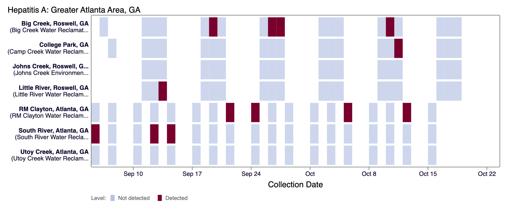
How do I interpret the heat maps?
The heat map show each site as a row, and each date as a column. The color blue means the sample was non-detect for the selected pathogen and white indicates no sample was collected on a particular day.
For Respiratory and Gastrointestinal pathogens, the colors get darker with higher wastewater concentrations.
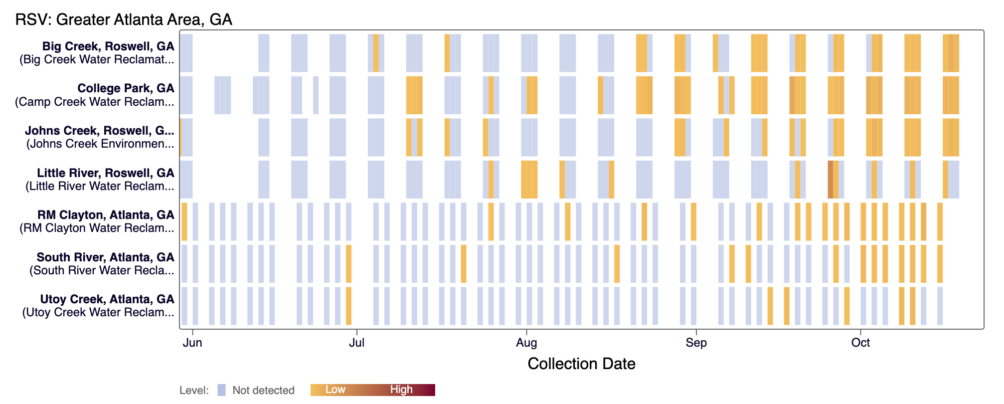
For Other (rarely detected) pathogens and H5 (influenza), the dark red color means there was a positive detection for the pathogen in that days sample.
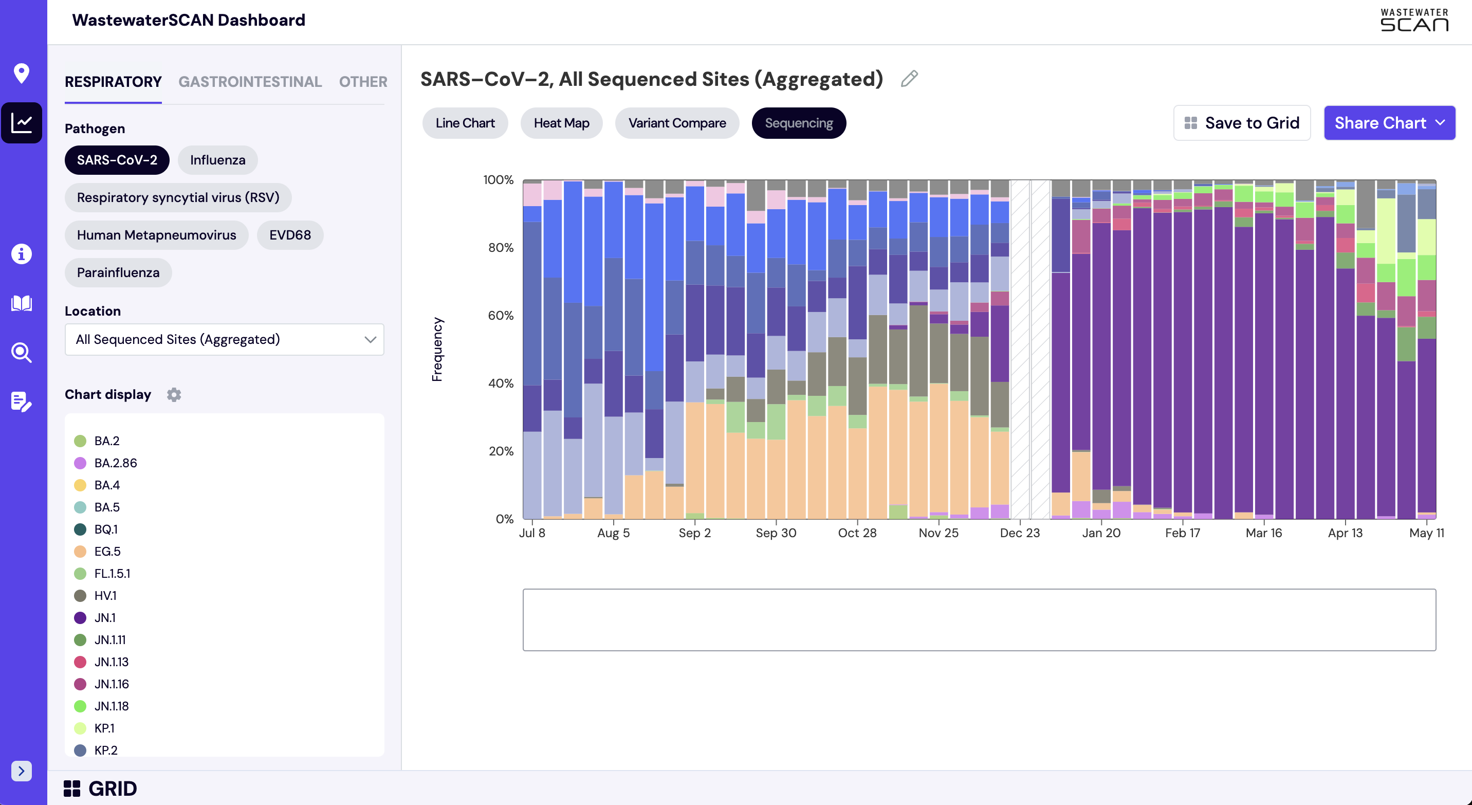
How do I interpret the sequencing charts?
The sequencing chart shows the relative proportions of different variants inferred from sequencing the entire genome of SARS-CoV-2. The different colors in the bar chart represent different variants. Results are based on sequencing of 2 samples per week, combined to provide a weekly value. The hashed gray bars indicate there is no data available for a given week. To learn more about the sequencing protocol, visit this link.
Note that the last processed sequencing data are always from samples taken between 1-2 weeks ago.
To see the national aggregated sequencing chart click here.
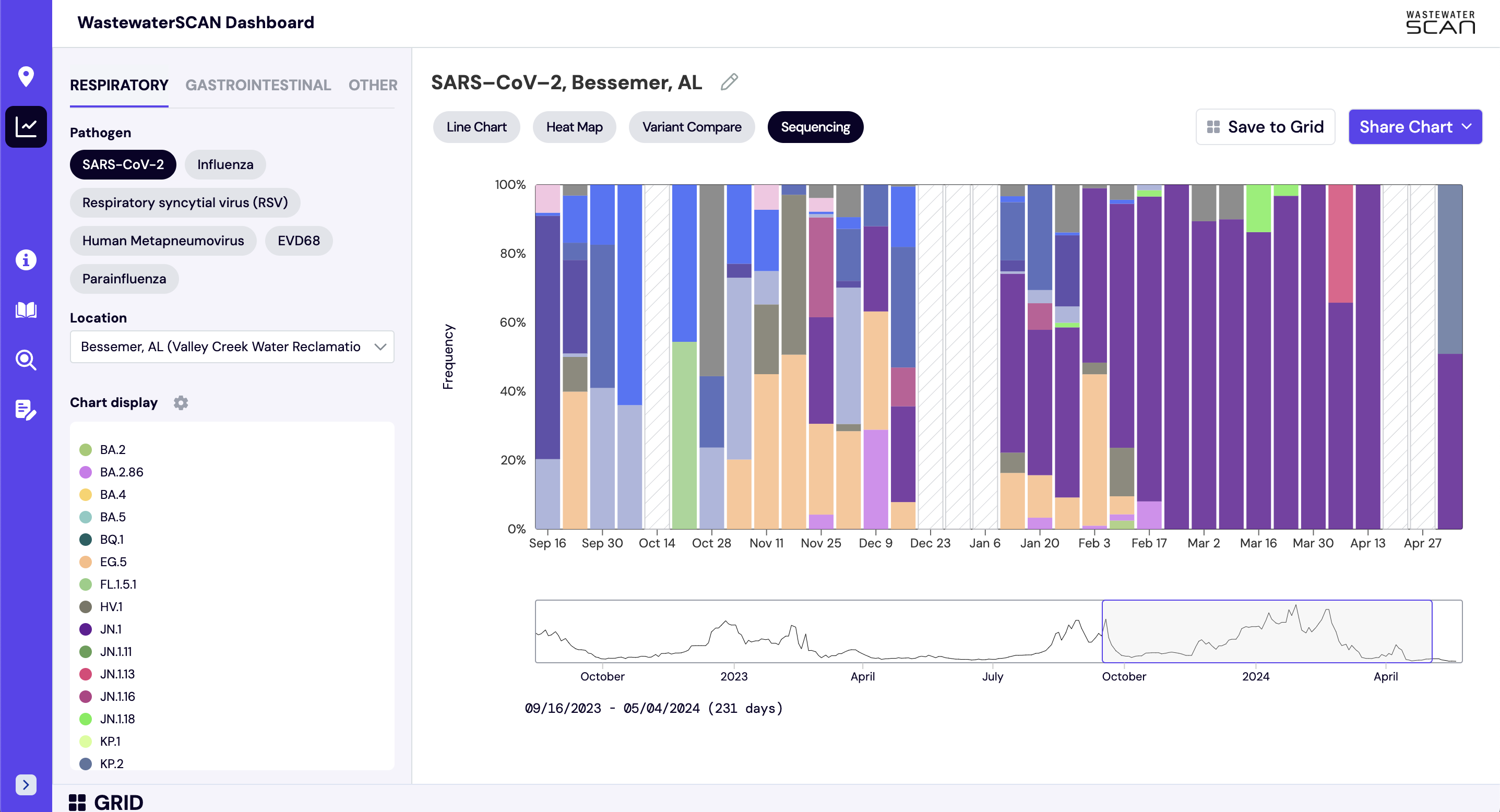
In the 'Chart' view:
- Select 'Respiratory' and 'SARS-CoV-2'
- Next search for one of the following sites in the 'Location' bar on the lefthand navigation panel: Bessemer, AL; Anchorage, AK; Oceanside, San Francisco, CA; Sacramento, CA; San Jose, CA; Southeast, San Francisco, CA; Washington, DC; North Miami, FL; Tallahassee, FL; College Park, GA; RM Clayton, Atlanta, GA; Sand Island, Honolulu, HI; West Boise, ID; Glen Ellyn, IL; South Bend, IN; Kaw Point, Kansas City, KS; Louisville, KY; Portland, ME; Hagerstown, MD; Boston, MA; Ann Arbor, MI; Rochester, MN; Theresa Street, Lincoln, NE; Las Vegas, NV; Newark, NJ; Youngstown, OH; Chester, PA; Garland, TX; South Laredo, TX; White Rock Central, Dallas, TX; Central Salt Lake Valley, UT.
- The 'Sequencing' button will now display above the chart on the right side of the screen. Click 'Sequencing' to display the stacked bar chart with variant data for the selected location.
How are aggregated trendlines determined?
Aggregated trend lines are population-weighted averages of data from groups of sites. These aggregated trend lines are available to view when a pre-existing group of sites is selected from the dropdown (i.e. a state, county, or other administrative area). The line can be optionally shown by clicking the “view” icon, and appears as a black line over data that is displayed for each of the individually selected sites. Aggregated trend lines are available for any target and any suggested set of site grouping. If you are interested in adding a custom group for an administrative area that you oversee, please contact us at wwscan_stanford_emory@lists.stanford.edu. These groups can be found under “Other Regions” when searching for locations.
Methodology: The aggregation approach depends on the geography. States and custom selections are aggregated using the population for each of the plants monitored. National and Regional groups are aggregated using the state and the population of each state monitored by WWSCAN (not the population monitored by WWSCAN in that state).
Aggregated trend lines for states and custom selections are calculated using the trimmed smoothed average for each site. For each date, an individual site trimmed smoothed value for the day is multiplied by the plant's population, then these are summed and divided by the total population of all selected sites. This calculation results in the trimmed weighted average target/PMMoVw,d for day d, as in the following equation for the X selected plants:

Prior to calculating the aggregated line, non-detect values are set to 500 cp/g (approximately half the limit of detection) / the average PMMoV value for the plant. Missing values are set using linear interpolation between the previous and next values with respect to the missing date.
Aggregated trend lines for the nation and regions are calculated using the trimmed smoothed average for each state included, as well as the total population from each state (not the individual plants). For each date, an individual state trimmed smoothed value for the day is multiplied by the population of the state, then these are summed and divided by the total population of all states in that region. This calculation results in the trimmed weighted average Target_w_trimmed_r,d for day d, as in the following equation for the S states in the region:
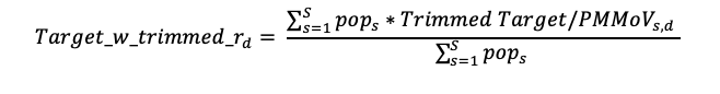
For data within the last 10 days, Target_w_trimmed_r,d should only be calculated when there is a value, either measured or interpolated, for 50% of the plants in the region.
How are national levels determined?
National levels shown on charts help to provide a relative interpretation of where current wastewater levels compare over the last 365 days. The national levels are available across all targets on the data.wastewaterscan.org platform.
The national levels are shown as groups (bottom, middle, and upper) that are based on looking back at all data from the last 365 days across all WWSCAN sites. The range of values included in the bottom third of all data points are represented by the bottom band, the range values included in the middle third of data points are represented by the middle band, and the range of values included in the top third of data points are represented as the top band. The lines denote the values at the 33rd and 66th percentiles. You may notice that the top third area often represents a larger range than the middle or bottom - this is because there is typically more variability in the concentrations in the top of third of data points.
- Lower third line: represents the area where the lower third (<33rd percentile) of the data for all WWSCAN sites falls.
- Middle third line: represents the area where the middle third (33rd - 66th percentile) of the data for all WWSCAN sites falls.
- Upper third line: represents the area where the upper third (>66th percentile) of the data for all WWSCAN sites falls.
The National Levels can be turned on by clicking the the 'National Levels' eye icon on the left hand navigation panel.
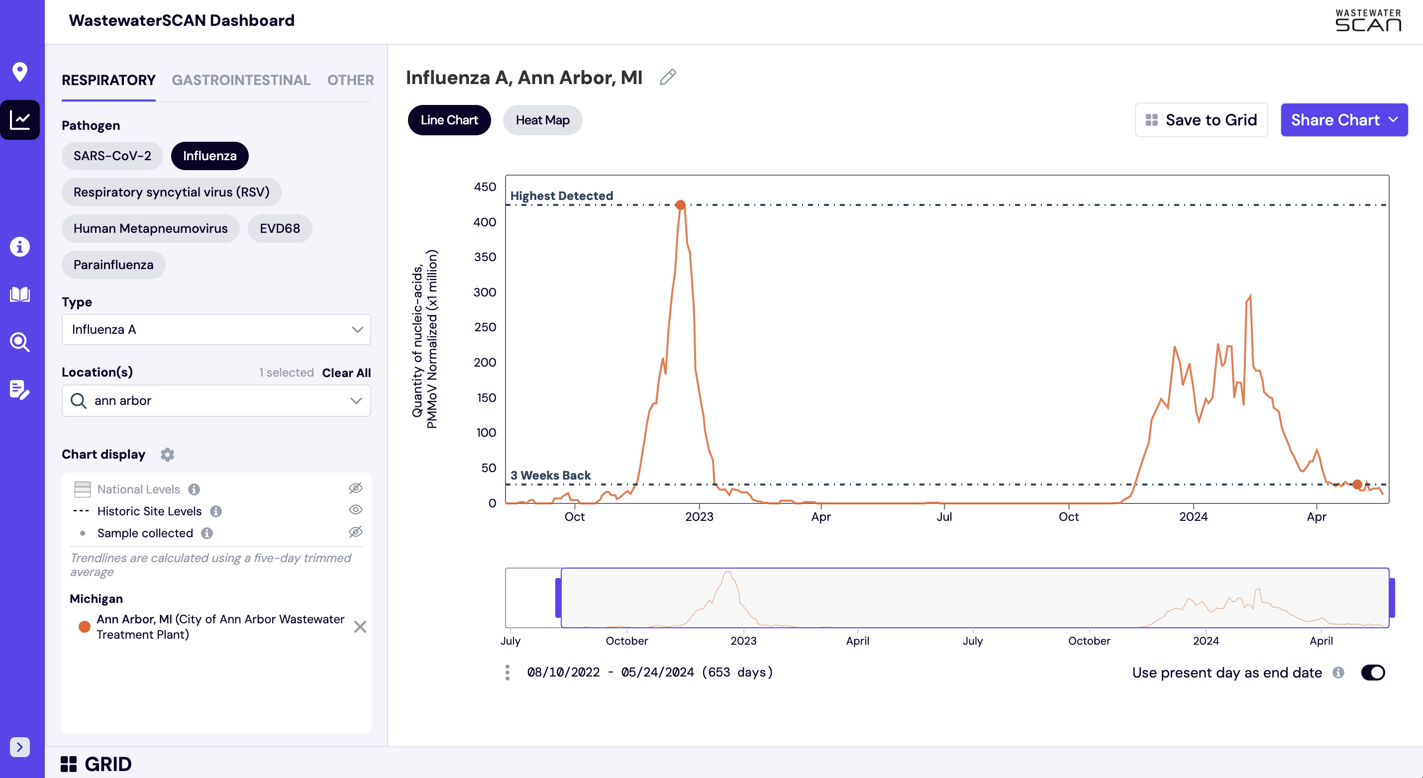
How are historical site levels determined?
Historic reference levels can be turned on for an individual site. The two reference lines that can be added to an individual site plot are ‘3 Weeks Back’ and ‘Highest Detected’ and these values are based on the smoothed, trimmed average values. These lines are used to provide context as to how the most recent sample compares to where wastewater levels were 3 weeks ago and the highest level detected at an individual site.
The ‘3 Weeks Back’ line helps the reader eye-ball if there has been an increase, decrease, or plateau in the previous 3 weeks. The ‘3 Weeks Back’ line also provides context as to roughly how much of an increase or decrease is observed. In the graph below, we can see the SARS-CoV-2 levels in Ann Arbor, MI had decreased from where they were 3 weeks ago.
The Historic reference levels can be turned on by clicking the the 'Historic Site Levels' eye icon on the left hand navigation panel.
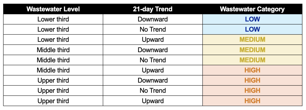
How are wastewater categories determined?
WastewaterSCAN uses a Wastewater Categorization system to communicate important insights from recent wastewater results. Research shows that the measurements we make in wastewater are related to disease in the community. The wastewater categorization helps us quickly understand if the recent measurements for a disease fall into a low, medium, or high category and are determined based on a combination of the following variables:
- Trends indicate how wastewater concentrations are changing over the last 21 days
- Levels indicate whether wastewater concentrations are relatively lower or higher
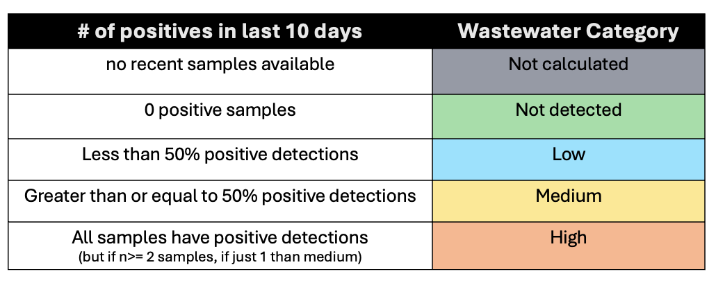
- Frequency of detection indicates how often a pathogen is detected in wastewater
It is important to note that if there is no sample in the system for the last 7 days, then a site gets a 'Not Calculated' flag due to limited data.
We are not currently calculating categories for human adenovirus group F, and the H1 & H3 influenza markers.
The Wastewater Categories are applied slightly differently for 3 archetypes of diseases:
1. Pathogens that are commonly detected (regardless of season) in wastewater → SARS-CoV-2, Norovirus, Rotavirus, and ‘peak season’ Respiratory pathogens (IAV, IBV, RSV, HMPV, EV-D68)
2. Seasonal pathogens (rarely detected outside of season/outbreaks) → IAV, IBV, RSV, HMPV, EV-D68
The methodology used to determine wastewater Onset vs wastewater Offset using raw target concentrations (not PMMoV Normalized) for individual sites is as follows
- The onset dates of IAV, RSV, HMPV, and EV-D68 wastewater events are identified as the first day for which all samples in a 14 day look back period had concentrations higher than or equal to 2,000 copies/g, which is approximately twice the lowest detectable concentration. Once IAV, RSV, HMPV, or EV-D68 are onset, the method for 'commonly detected pathogens' (see above) is used to determine the wastewater categorization.
- The offset dates of IAV, RSV, HMPV, and EV-D68 wastewater events were identified as the first day after a wastewater onset event for which only 50% of samples during a 14-d look back period have concentrations higher than or equal to 2,000 copies/g. When one of these signals is in offset, it is assign a ‘LOW’ categorization.
3. Pathogens that are not commonly detected (regardless of season) in wastewater →Candidozyma auris, Hepatitis A, H5 influenza marker, Measles, Mpox clade Ib, Mpox clade II, Parvovirus, and West Nile Virus
The methodology requires at least 21 days of data to calculate a category.
How do I interpret SARS-CoV-2 variant results?
SARS-CoV-2 variants are monitored using digital PCR by targeting a section of the genome that is specific to that variant or a small group of variants. It should be noted that the mutations we measure that are found in variants of SARS-CoV-2 are sometimes also found in other variants, so the presence of the mutation in wastewater does not provide certainty that the particular variant is present. Rather, the presence of the mutation suggests that the presence of the variant is possible but does not rule out the presence of the mutation contributed from other variant genomes. This link provides a detailed description of considerations when attempting variant detection in wastewater either through sequencing or targeted PCR-based assays. However, our research suggests that the concentrations of characteristic mutations of variants of concerns is strongly associated with the fraction of clinical cases that are sequenced and assigned to the variant.
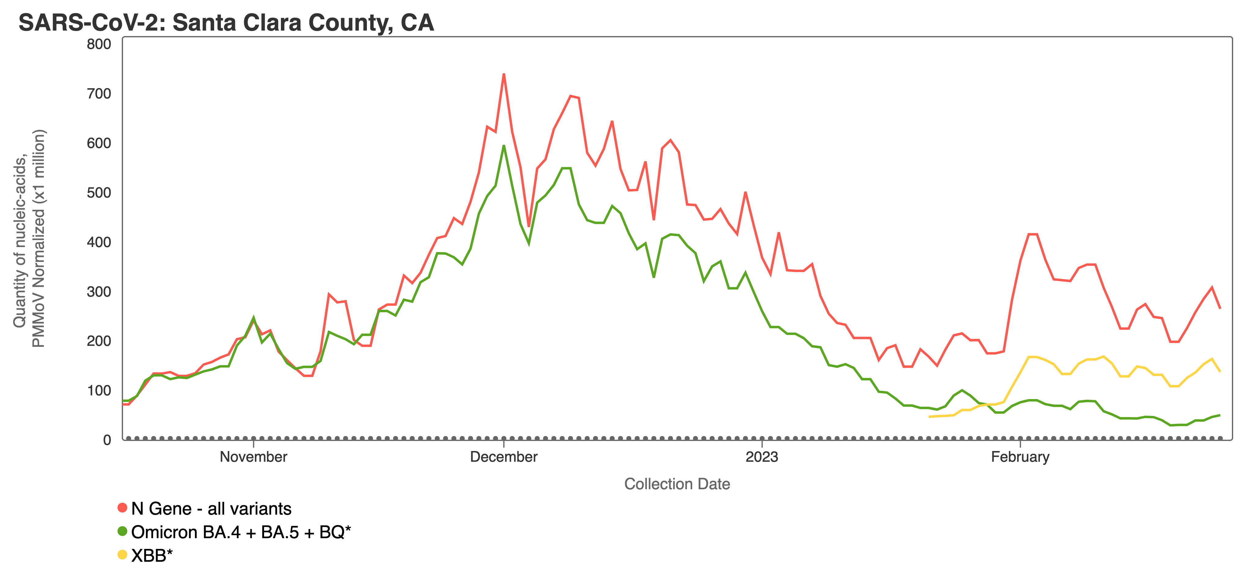
Variants can be viewed together for a single site using the “View by Variant” tab when making charts with SARS-CoV-2 on the website (screenshot below). The screenshot above shows the N gene (total SARS-CoV-2) concentration in red, with BA.4/BA.5/BQ in green and XBB* in yellow. You can observe that the concentration of BA.4/BA.5/BQ decreases in comparison to the N gene, while the XBB* target concentration appears to rise closer to the N gene concentration. This can be interpreted to mean that more of the SARS-CoV-2 genomes in wastewater solids from this site have the XBB* mutations than the mutation characteristic of the BA.4, BA.5, and BQ* variants. This is consistent with what we know from sequencing of clinical specimens, which shows that during the time depicted XBB* (and XBB 1.5 in particular) is replacing other variants.
How do I interpret the Influenza subtype results?
To compare the Influenza subtypes as a line chart, switch ‘View By’ from Location to Subtype. Next, select your desired site in the ‘Location’ dropdown. For the Subtype view you can only look at one site at a time.
Click on the gear icon in the ‘Chart display’ section to switch off ‘Show trendlines’ and ‘normalized by PMMoV’ and switch on ‘Show raw data points’. Now you can click the eye icons next to ‘Influenza A’, 'H1', 'H3’, and 'H5’ to display the data in the chart. You can hover over an individual point to get the concentration value as copies per gram.


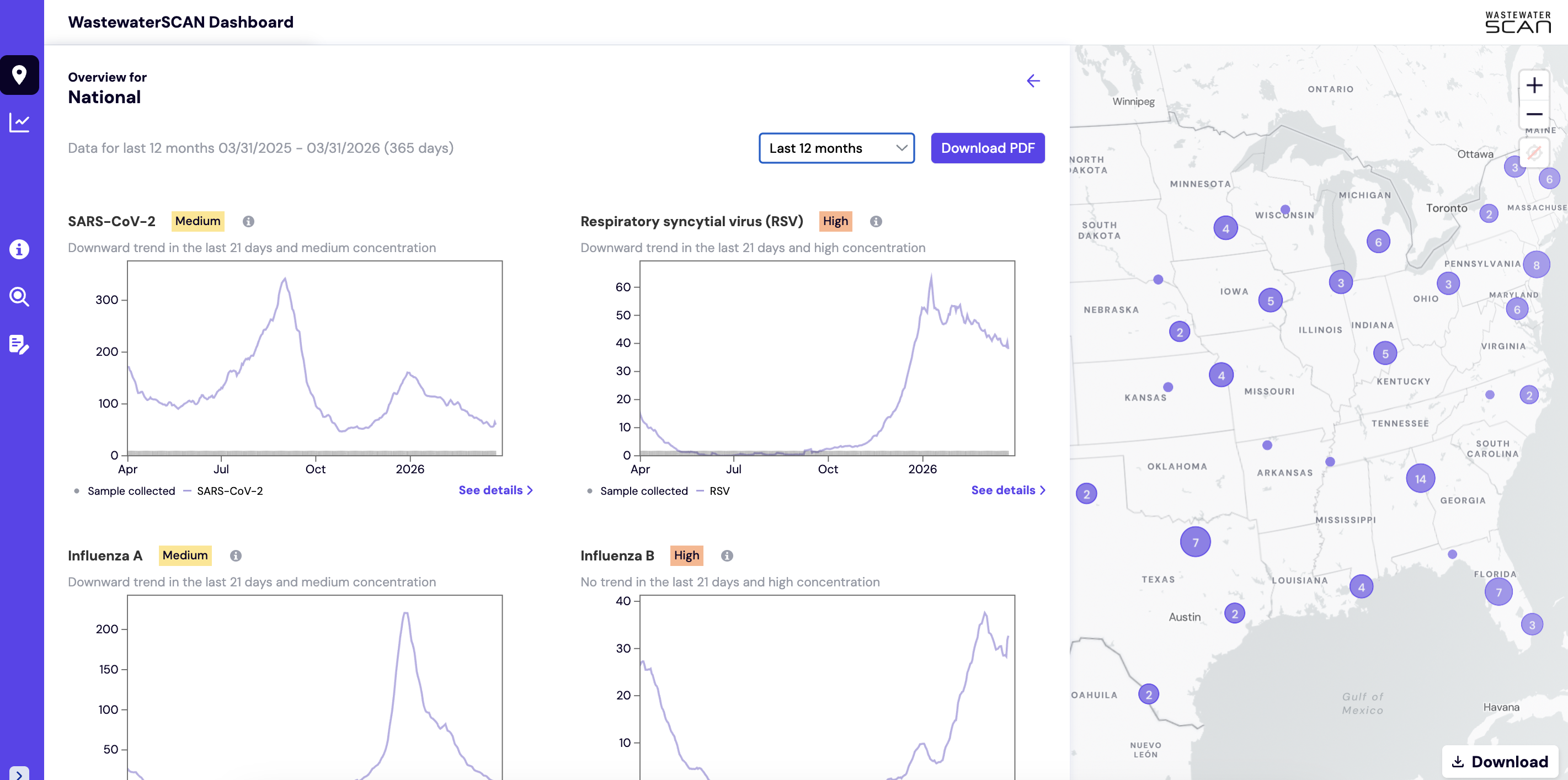
Where can I find the National and Regional trends for WastewaterSCAN sites?
The National and Regional overview summary shows the levels of SARS-CoV-2, Influenza A, Influenza B, Respiratory syncytial virus, Human metapneumovirus, Mpox clade II, Norovirus, Rotavirus, Enterovirus D68, Candia auris, and Hepatitis A detected in wastewater samples across WastewaterSCAN sites.
- WWSCAN Main Overview panel: here
- WWSCAN National Overview:here
- WWSCAN Midwest Overview: here
- WWSCAN Northeast Overview: here
- WWSCAN South Overview: here
- WWSCAN West Overview: here
All charts show quantity of nucleic-acids, PMMoV Normalized (x1 million). The charts default to show the last 3 months but from the dropdown you can select a length of time from the following four options: last 6 weeks, last 3 months, last 6 months, last 12 months, last 24 months). These Overview charts can be downloaded as PDF to share.
How are samples collected?
Wastewater is collected from wastewater treatment plants by staff and shipped to our partner lab at Verily. Samples of either liquid influent wastewater or settled solids from a primary clarifier are taken, and then the solids from these samples are utilized for analysis. Samples from primary clarifiers are usually “grab” samples taken at one point in time, but we note that these are in fact solids from the wastewater that are collected over many hours in the clarifiers. They are therefore essentially a composite of wastewater solids from the community over several hours. Influent samples that are submitted are composite samples. All samples are held at 4°C prior to analysis. Shipping materials are provided to plants, and samples are shipped overnight on ice.
How are samples analyzed?
At the lab, samples are processed for genomic targets for the pathogens that WastewaterSCAN tests for. One strength of the program is the ability to add (and occasionally subtract) targets for analysis. Using the solids from wastewater and using consistent methods across our sites nationally helps us produce consistent, comparable data from across the United States.Pre-analytical steps are the same for all targets and digital PCR assays can be added in multiplex.
Pre-analytical steps: Solids are dewatered into a thick pellet by centrifuging at high speeds. If necessary, solids from an influent sample can first be thickened by settling in an imhoff cone. After solids have been dewatered, a small aliquot is resuspended in a buffer solution and homogenized. This solution is then spun down, and the supernatant is used for further analysis. Prior to nucleic acid extraction, samples are spiked with a vaccine strain of bovine coronavirus (BCoV) to measure the recovery of BCoV in each sample.
Protocol:
- Aaron Topol, Marlene Wolfe, Brad White, Krista Wigginton, Alexandria B Boehm 2021. High Throughput pre-analytical processing of wastewater settled solids for SARS-CoV-2 RNA analyses. protocols.io Link.
DNA/RNA extraction: The buffer solution supernatant from the pre-analytical steps is then used for DNA/RNA extraction using the Chemagic 360. An inhibitor removal step is also used.
Protocol:
- Aaron Topol, Marlene Wolfe, Krista Wigginton, Bradley White, Alexandria B Boehm 2021. High Throughput RNA Extraction and PCR Inhibitor Removal of Settled Solids for Wastewater Surveillance of SARS-CoV-2 RNA. protocols.io Link
ddPCR analysis: Target genes specific to each pathogen are measured using RT droplet digital PCR. Results are reported as copies per dry weight of solids. Additionally, we measure pepper mild mottle virus (PMMoV) as an internal control and results for this target are reported per gram dry weight. We estimate that the limit of detection for these assays is typically about 1000 cp/g.
Protocols:
- Aaron Topol, Marlene Wolfe, Brad White, Krista Wigginton, Alexandria B. Boehm. 2021. High Throughput SARS-COV-2, PMMOV, and BCoV quantification in settled solids using digital RT-PCR. protocols.io Link.
- Bridgette Hughes, Brad White, Marlene Wolfe, Alexandria Boehm 2021. Quantification of SARS-CoV-2 variant mutations (HV69-70, E484K/N501Y, del156-157/R158G, del143-145, LPPA24S) in settled solids using digital RT-PCR. protocols.io Link.
- Bridgette Hughes, Brad White, Marlene Wolfe, Krista Wigginton, Alexandria Boehm 2021. B. Hughes, B. J. White, M. K. Wolfe, A. B. Boehm. 2022.Quantification of various SARS-CoV-2 variant mutations (characteristic of Alpha, Beta, Gamma, Delta, Omicron and Omicron sublineages) in settled solids using digital RT-PCR . protocols.io Link.
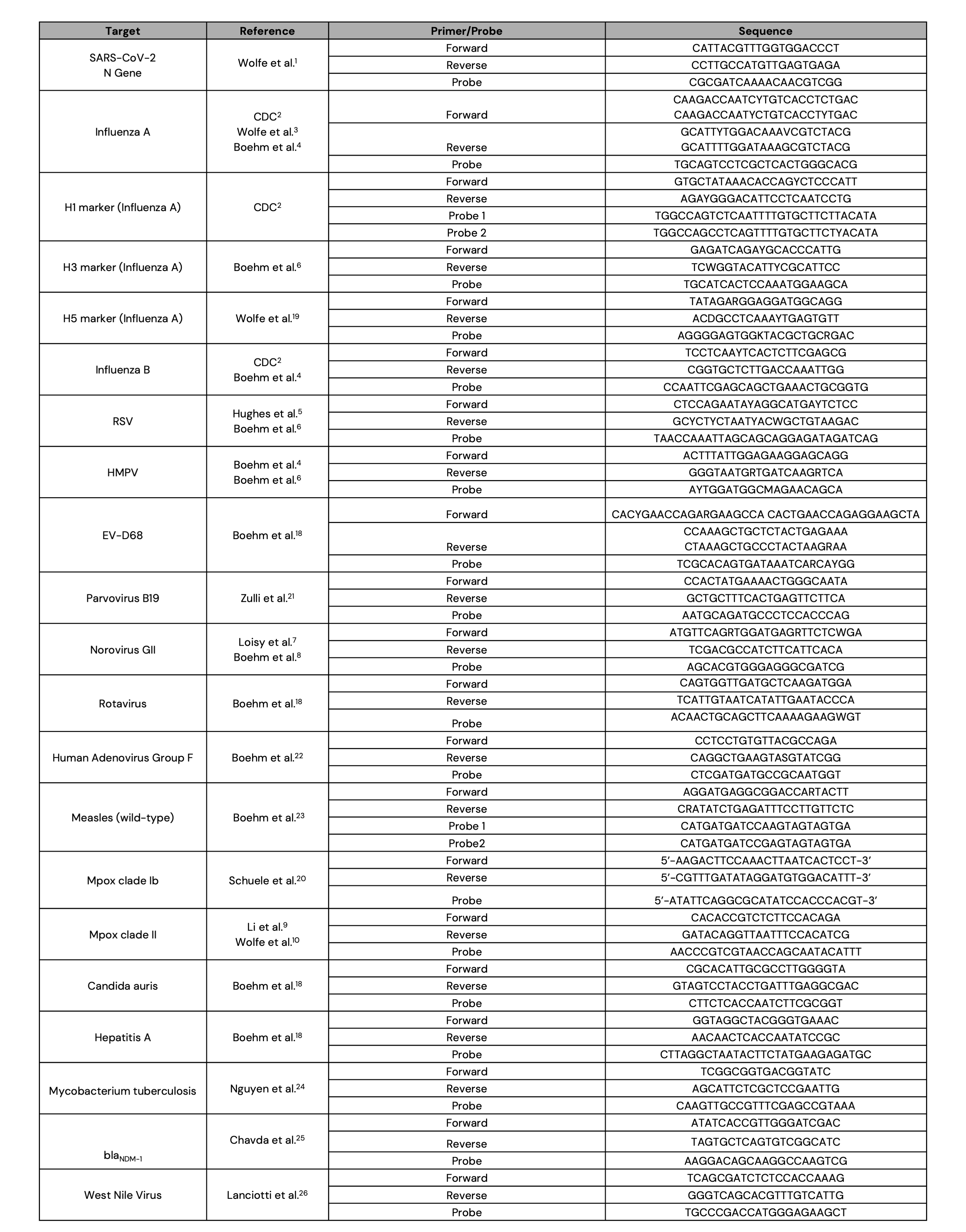
WastewaterSCAN is currently utilizing the following targets for the diseases we monitor:
Main Disease Targets
Controls
References:
- Wolfe, M. K.; Topol, A.; Knudson, A.; Simpson, A.; White, B.; Duc, V.; Yu, A.; Li, L.; Balliet, M.; Stoddard, P.; Han, G.; Wigginton, K. R.; Boehm, A. High-Frequency, High-Throughput Quantification of SARS-CoV-2 RNA in Wastewater Settled Solids at Eight Publicly Owned Treatment Works in Northern California Shows Strong Association with COVID-19 Incidence. mSystems 2021, 6 (5), e00829-21. https://doi.org/10.1128/mSystems.00829-21.
- United States Center for Disease Control. Research Use Only CDC Flu SC2 Multiplex Assay Primers and Probes. https://www.cdc.gov/coronavirus/2019-ncov/lab/multiplex-primer-probes.html (accessed 2022-08-18).
- Wolfe, M. K.; Duong, D.; Bakker, K. M.; Ammerman, M.; Mortenson, L.; Hughes, B.; Arts, P.; Lauring, A. S.; Fitzsimmons, W. J.; Bendall, E.; Hwang, C. E.; Martin, E. T.; White, B. J.; Boehm, A. B.; Wigginton, K. R. Wastewater-Based Detection of Two Influenza Outbreaks. Environ. Sci. Technol. Lett. 2022. https://doi.org/10.1021/acs.estlett.2c00350.
- Boehm, A. B.; Hughes, B.; Duong, D.; Chan-Herur, V.; Buchman, A.; Wolfe, M. K.; White, B. J. Wastewater Concentrations of Human Influenza, Metapneumovirus, Parainfluenza, Respiratory Syncytial Virus, Rhinovirus, and Seasonal Coronavirus Nucleic-Acids during the COVID-19 Pandemic: A Surveillance Study. Lancet Microbe 2023, 0 (0). https://doi.org/10.1016/S2666-5247(22)00386-X.
- Hughes, B.; Duong, D.; White, B. J.; Wigginton, K. R.; Chan, E. M. G.; Wolfe, M. K.; Boehm, A. B. Respiratory Syncytial Virus (RSV) RNA in Wastewater Settled Solids Reflects RSV Clinical Positivity Rates. Environ. Sci. Technol. Lett. 2022, 9 (2), 173–178. https://doi.org/10.1021/acs.estlett.1c00963.
- Boehm, A. B.; Wolfe, M. K.; White, B. J.; Hughes, B.; Duong, D.; Bidwell, A. More than a Tripledemic: Influenza A Virus, Respiratory Syncytial Virus, SARS-CoV-2, and Human Metapneumovirus in Wastewater during Winter 2022–2023. Environ. Sci. Technol. Lett. 2023, 10 (8), 622–627. https://doi.org/10.1021/acs.estlett.3c00385.
- Loisy, F.; Atmar, R. L.; Guillon, P.; Le Cann, P.; Pommepuy, M.; Le Guyader, F. S. Real-Time RT-PCR for Norovirus Screening in Shellfish. J. Virol. Methods 2005, 123 (1), 1–7. https://doi.org/10.1016/j.jviromet.2004.08.023.
- Boehm, A. B.; Wolfe, M. K.; White, B. J.; Hughes, B.; Duong, D.; Banaei, N.; Bidwell, A. Human Norovirus (HuNoV) GII RNA in Wastewater Solids at 145 United States Wastewater Treatment Plants: Comparison to Positivity Rates of Clinical Specimens and Modeled Estimates of HuNoV GII Shedders. J. Expo. Sci. Environ. Epidemiol. 2023, 1–8. https://doi.org/10.1038/s41370-023-00592-4.
- Li, Y.; Zhao, H.; Wilkins, K.; Hughes, C.; Damon, I. K. Real-Time PCR Assays for the Specific Detection of Monkeypox Virus West African and Congo Basin Strain DNA. J. Virol. Methods 2010, 169 (1), 223–227. https://doi.org/10.1016/j.jviromet.2010.07.012.
- Wolfe, M. K.; Yu, A. T.; Duong, D.; Rane, M. S.; Hughes, B.; Chan-Herur, V.; Donnelly, M.; Chai, S.; White, B. J.; Vugia, D. J.; Boehm, A. B. Use of Wastewater for Mpox Outbreak Surveillance in California. N. Engl. J. Med. 2023. https://doi.org/10.1056/NEJMc2213882.
- Yu, A.; Hughes, B.; Wolfe, M.; Leon, T.; Duong, D.; Rabe, A.; Kennedy, L.; Ravuri, S.; White, B.; Wigginton, K. R.; Boehm, A.; Vugia, D. Estimating Relative Abundance of Two SARS-CoV-2 Variants through Wastewater Surveillance at Two Large Metropolitan Sites. Emerg. Infect Dis 2022, 28 (5), 940–947.
- Wolfe, M.; Hughes, B.; Duong, D.; Chan-Herur, V.; Wigginton, K. R.; White, B. J.; Boehm, A. B. Detection of SARS-CoV-2 Variants Mu, Beta, Gamma, Lambda, Delta, Alpha, and Omicron in Wastewater Settled Solids Using Mutation-Specific Assays Is Associated with Regional Detection of Variants in Clinical Samples. Appl. Environ. Microbiol. 2022, 88 (8), e00045-22. https://doi.org/10.1128/aem.00045-22.
- Hughes, B.; White, B. J.; Wolfe, M. K.; Boehm, A. B. Quantification of SARS-CoV-2 Variant Mutations (HV69-70, E484K/N501Y, Del156-157/R158G, Del143-145, LPPA24... 2022.
- Decaro, N.; Elia, G.; Campolo, M.; Desario, C.; Mari, V.; Radogna, A.; Colaianni, M. L.; Cirone, F.; Tempesta, M.; Buonavoglia, C. Detection of Bovine Coronavirus Using a TaqMan-Based Real-Time RT-PCR Assay. J. Virol. Methods 2008, 151 (2), 167–171. https://doi.org/10.1016/j.jviromet.2008.05.016.
- Graham, K. E.; Loeb, S. K.; Wolfe, M. K.; Catoe, D.; Sinnott-Armstrong, N.; Kim, S.; Yamahara, K. M.; Sassoubre, L. M.; Mendoza Grijalva, L. M.; Roldan-Hernandez, L.; Langenfeld, K.; Wigginton, K. R.; Boehm, A. B. SARS-CoV-2 RNA in Wastewater Settled Solids Is Associated with COVID-19 Cases in a Large Urban Sewershed. Environ. Sci. Technol. 2021, 55 (1), 488–498. https://doi.org/10.1021/acs.est.0c06191.
- Haramoto, E.; Kitajima, M.; Kishida, N.; Konno, Y.; Katayama, H.; Asami, M.; Akiba, M. Occurrence of Pepper Mild Mottle Virus in Drinking Water Sources in Japan. Appl. Environ. Microbiol. 2013, 79 (23), 7413–7418. https://doi.org/10.1128/AEM.02354-13.
- Zhang, T.; Breitbart, M.; Lee, W. H.; Run, J.-Q.; Wei, C. L.; Soh, S. W. L.; Hibberd, M. L.; Liu, E. T.; Rohwer, F.; Ruan, Y. RNA Viral Community in Human Feces: Prevalence of Plant Pathogenic Viruses. PLoS Biol. 2006, 4 (1), e3. https://doi.org/10.1371/journal.pbio.0040003.
- Boehm, A., Wolfe, M. K., White, B., Hughes, B., & Duong, D. (2023). Two years of longitudinal measurements of human adenovirus group F, norovirus GI and GII, rotavirus, enterovirus, enterovirus D68, hepatitis A virus, Candida auris, and West Nile virus nucleic-acids in wastewater solids: A retrospective study at two wastewater treatment plants. medRxiv, 2023-08.
- Wolfe, M.K., Duong, D., Shelden, B., Chan, E.M., Chan-Herur, V., Hilton, S., Paulos, A.H., Xu, X.R.S., Zulli, A., White, B.J. and Boehm, A.B., 2024. Detection of hemagglutinin H5 influenza A virus sequence in municipal wastewater solids at wastewater treatment plants with increases in influenza A in spring, 2024. Environmental science & technology letters, 11(6), pp.526-532.
- Schuele, L.; Masirika, L. M.; Udahemuka, J. C.; Siangoli, F. B.; Mbiribindi, J. B.; Ndishimye, P.; Aarestrup, F. M.; Koopmans, M.; Munnink, B. B. O.; Molenkamp, R.; Group, G. M. Real-Time PCR Assay to Detect the Novel Clade Ib Monkeypox Virus, September 2023 to May 2024. Eurosurveillance 2024, 29 (32), 2400486.
- Zulli, A., Linfield, R. Y., Duong, D., Hughes, B., & Boehm, A. B. (2025). Community infections linked with parvovirus B19 genomic DNA in Wastewater, Texas, USA, 2023–2024. Emerging Infectious Diseases, 31(7), 1442.
- Boehm AB, Shelden B, Duong D, Banaei N, White BJ, Wolfe MK.2024.A retrospective longitudinal study of adenovirus group F, norovirus GI and GII, rotavirus, and enterovirus nucleic acids in wastewater solids at two wastewater treatment plants: solid-liquid partitioning and relation to clinical testing data. mSphere9:e00736-23.https://doi.org/10.1128/msphere.00736-23
- Boehm, A. B., Wolfe, M. K., Bidwell, A. L., Zulli, A., White, B. J., Shelden, B., & Duong, D. (2026). Pathogen nucleic acids data in wastewater solids from 147 treatment plants in the United States: 2024-2025. Data in Brief, 112503.
- Nguyen T, Mercier E, Wong CH, Hegazy N, Kabir MP, Tomalty E, Addo F, Ward L, Renouf E, Wan S, Tcholakov Y, Guilherme S, Delatolla R. Partitioning and probe-based quantitative PCR assays for the wastewater monitoring of Mycobacterium tuberculosis complex, M. tuberculosis, and M. bovis. J Water Health. 2025 Oct;23(10):1163-1179. doi: 10.2166/wh.2025.102. Epub 2025 Sep 19. PMID: 41170952.
- Chavda KD, Satlin MJ, Chen L, Manca C, Jenkins SG, Walsh TJ, Kreiswirth BN.2016.Evaluation of a Multiplex PCR Assay To Rapidly Detect Enterobacteriaceae with a Broad Range of β-Lactamases Directly from Perianal Swabs. Antimicrob Agents Chemother60:.https://doi.org/10.1128/aac.01458-16
- Lanciotti RS, Kerst AJ, Nasci RS, Godsey MS, Mitchell CJ, Savage HM, Komar N, Panella NA, Allen BC, Volpe KE, Davis BS, Roehrig JT.2000.Rapid Detection of West Nile Virus from Human Clinical Specimens, Field-Collected Mosquitoes, and Avian Samples by a TaqMan Reverse Transcriptase-PCR Assay. J Clin Microbiol38:.https://doi.org/10.1128/jcm.38.11.4066-4071.2000
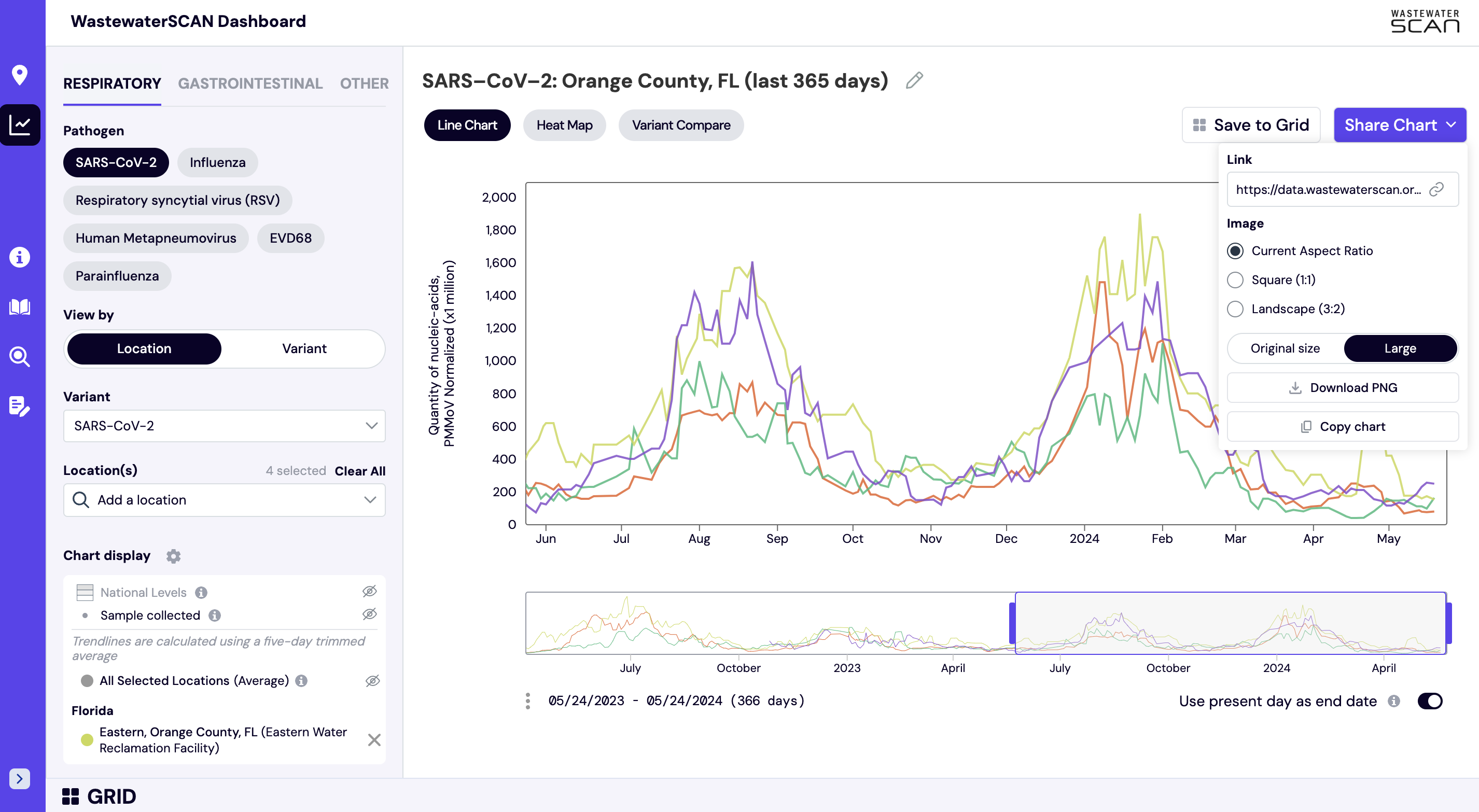
How can I download and share this chart?
When viewing a chart on the website, you can share or download the chart by selecting the purple "Share Chart" button (see below). The chart can be shared by downloading the image or copying a link directly to your selections.
Data license
Content on this site is licensed under CC BY-NC 4.0.
Data information and use
These data were generated by the WastewaterSCAN / SCAN projects, philanthropically funded through a gift to Stanford University. All results are understood to be based on inputs that are experimental in nature, and are not intended to diagnose or treat any disease. The results are provided “as is” and without warranty of any kind. Stanford is not liable for any claim arising out of or in connection with the disclosure of these results. By accessing or copying any part of the database, the user accepts the terms of this license.
These data are being made available to inform public health decision making. Anyone seeking to use the database for other purposes or for research is required to contact the WastewaterSCAN / SCAN team at wwscan_stanford_emory@lists.stanford.edu or Alexandria Boehm aboehm@stanford.edu. Any questions about the data, or the methods used to generate or produce any data products should be directed to the same emails.
When the data are used in any format, the following attribution should be made: “These data were collected as part of the WastewaterSCAN / SCAN project, a partnership between Stanford University, Emory University, and Verily funded philanthropically through a gift to Stanford University.” In addition, the following paper should be cited:
- A. B. Boehm, M. K. Wolfe, A. L. Bidwell, A. Zulli, B. J. White, B. Shelden, D. Duong. Pathogen nucleic acids data in wastewater solids from 147 treatment plants in the United States: 2024-2025. Data in Brief, 2026. Link to paper.
It should be noted that the required attribution may change over time and users should check back here often to conform to the requirements.
WWSCAN Peer-Reviewed Scientific Publications
You can find a complete list of peer-reviewed publications utilizing the WWSCAN data here.
WWSCAN newsletter & blog
To stay up-to-date on current wastewater trends and levels, you can find WWSCAN's monthly newsletter here: https://wwscan.ghost.io/
You can find a complete catalog of WWSCAN's achieved newsletters and blog posts here: https://wwscan.ghost.io/page/2/